Train how-to
Summary
The train tool performs the training loop of a segmentation model. As for now, only 3 models are implemented :
classic U-Net
a light version of the standard Unet with much less parameter
U-Net with ResNet as backbone
Deeplabv3+ (with MobileNetV2 as backbone)
Basic U-Net is available in 2 versions, a [lighter version](#light-u-net) with less feature channels and the [original one](#u-net). Torchvision implementations of MobileNetV2 has been adapted to accept input images with more than 3 channels.
The main inputs of the training step are:
description of data sources: csv files for train dataset and optionnaly for validation dataset. Those files must describe each tuple image/label files
Example of csv file
/path/to/dataset/train/img/15-7826_4-2467_0.tif,/path/to/dataset/train/msk/15-7826_4-2467_0.tif
/path/to/dataset/train/img/15-7586_4-2492_1.tif,/path/to/dataset/train/msk/15-7586_4-2492_1.tif
/path/to/dataset/train/img/15-8091_4-2272_3.tif,/path/to/dataset/train/msk/15-8091_4-2272_3.tif
/path/to/dataset/train/img/15-8038_4-2541_4.tif,/path/to/dataset/train/msk/15-8038_4-2541_4.tif
description of model: name of the model, output folder to write checkpoints and history.
setup of the training: hyperparameters
The train stops when a patience criteria has been reached: if the loss calculated on validation dataset does not decrease during a number of epochs, the training loop stops. The default number of epochs to wait for model improvement is set to 20.
The train tool is called like this:
$ odeon train -c /path/to/my/json/config/file/my_json_config_file.json
A -v option is available for debug, using it increases the training time because it activates the computation of IOU for each training batches.
Configuration
The json configuration file in input of CLI command contains 3 sections:
Data source
train_file (string): path to the CSV file of the train datasetval_file (string, optional): path to the CSV file of the validation datasetpercentage_val (float, optional): ifval_fileis not specified, a percentage of the train dataset is used for validationimage_bands (list of integer, optional): a list of band indices. Only specified bands of input images will be used in training. All bands are used by default.mask_bands (list of integer, optional): a list of band indices. Only specified bands of input masks will be used in training. All bands are used by default.
Model setup
model_name (string): name of model to train (values available: ‘unet’, ‘lightunet’, ‘resnet18’, ‘resnet34’, ‘resnet50’, ‘resnet101’, ‘resnet150’,’deeplab’). See [Model description](#model-description).output_folder (string): path to output folder. Model file and training curves with loss and IOU are stored by default. If save_history is set to true in train_setup section, a json file with values by epoch is saved.model_filename (string, optional): name of model file. Two files are saved during training: ${model_filename}.pth and optimizer_${model_filename}.pth in order to store the state_dict of model and optimizer. When model improves, files are overwritten. By default, model_filename=${model_name}.pth.
Train setup
epochs (integer, optional, default 300): number of epochs.batch_size (integer, optional, default 16): size of training batchespatience (integer default 20): number of epochs of no improvement to wait before stopping the training.save_history (boolean, optional, default false): flag to activate the saving of history. See History File Description.continue_training (boolean, optional, default false: tag to resume an interrupted training. Model and training metadata are saved on files with LAST prefix if training is stopped because of early_stopping (patience) or number of epochs conditions. In case of unwanted training stopping (Ctrl-C /keyboard interrupted) models and training information are saved into files with INTERUPTED prefix. Training is recover from the last modified models files.loss (string, optional, default "ce"): loss function, see Losses description.class imbalance (list of float, optional): a list of weights for each class. Usable only when loss is set to ce.optimizer (string, optional, default "adam"):optimizer, see Optimizer description.
lr (number, optional, default 0.001): starting learning rate. ` ReduceLROnPlateau <https://pytorch.org/docs/stable/optim.html?highlight=reducelronplateau#torch.optim.lr_scheduler.ReduceLROnPlateau>`_ is used as learning rate scheduler with mode=’min’, factor=0.5, patience=10, min_lr=1e-7, cooldown=4.data_augmentation (Union(string, array), default: ["rotation90"]: data augmentation transforms, see Augmentation description.device (string, optional): name of device used for training. If device is not specified and GPU is available, ‘cuda’ will be used, otherwise ‘cpu’. It can be usefull when multiple GPU is available (set to cuda:0, cuda:1, …).
Here is a minimal (without optional parameters set to default) and a full example of a configuration file needed for train process:
Minimal configuration file
{
      "data_source": {
          "train_file": "/path/to/train/csv/file.csv",
          "percentage_val": 0.2
      },
      "model_setup": {
          "model_name": "deeplab",
          "output_folder": "/path/to/output/folder",
          "model_filename": "deeplab.pth"
      }
}
Full configuration file
{
     "data_source": {
        "train_file": "/path/to/train/csv/file.csv",
        "val_file": "/path/to/validation/csv/file.csv",
        "image_bands": [1, 2, 3],
        "mask_bands": [2, 3, 7]
     },
     "model_setup": {
        "model_name": "deeplab",
        "output_folder": "/path/to/output/folder",
        "model_filename": "deeplab.pth"
     },
     "train_setup": {
        "epochs": 150,
        "batch_size": 8,
        "patience": 10,
        "save_history": true,
        "continue_training": true,
        "loss": "ce",
        "class_imbalance": [8.33, 3.57, 5, 50],
        "optimizer": "SGD",
        "lr": 0.005,
        "data_augmentation": ["rotation90", "radiometry"],
        "device": "cuda:0",
        "reproducible": false
     }
}
Model description
U-Net
{
  "model": "unet"
}
The original U-Net (` U-Net: Convolutional Networks for Biomedical Image Segmentation <https://arxiv.org/abs/1505.04597>`_)implementation.
# encoder
self.inc = InputConv(n_channels, 64, batch_norm=True)
self.down1 = EncoderConv(64, 128, batch_norm=True)
self.down2 = EncoderConv(128, 256, batch_norm=True)
self.down3 = EncoderConv(256, 512, batch_norm=True)
self.down4 = EncoderConv(512, 1024, batch_norm=True)
# decoder
self.up1 = DecoderConv(1024, 512, batch_norm=True)
self.up2 = DecoderConv(512, 256, batch_norm=True)
self.up3 = DecoderConv(256, 128, batch_norm=True)
self.up4 = DecoderConv(128, 64, batch_norm=True)

# last layer
self.outc = OutputConv(64, n_classes)
Light U-Net
{
     "model": "lightunet"
}
A light implementation of original U-Net with a small number of feature channels model is used here.
# encoder
self.inc = InputConv(n_channels, 8)
self.down1 = EncoderConv(8, 16)
self.down2 = EncoderConv(16, 32)
self.down3 = EncoderConv(32, 64)
self.down4 = EncoderConv(64, 128)
# decoder
self.up1 = DecoderConv(128, 64)
self.up2 = DecoderConv(64, 32)
self.up3 = DecoderConv(32, 16)
self.up4 = DecoderConv(16, 8)

# last layer
self.outc = OutputConv(8, n_classes)
U-Net + ResNet
{
 "model": ["resnet18", "resnet34", "resnet50", "resnet101", "resnet152"]
}
U-Net model using ResNet (18, 34, 50, 101 or 152) encoder.
The torchvision resnet implementation is reused here as encoder of a U-Net shaped network. The first convolutional layer is overwritten to fit the number of input channels of the images (which can be greater than 3).
An option is available in model constructor to use wether a bilinear interpolation (nn.Upsample with scale_factor=2) or a deconvolution (nn.ConvTranspose2d with stride=2) in decoder layers.
DeeplabV3+
{
   "model": "deeplab"
}
The DeeplabV3+ model is built from DeeplabV3 modules available in torchvision.
The implementation is inspired by what has been done in tensorflow
def __init__(self, n_channels, n_classes, output_stride=8):
   ...
   self.backbone = MobileNetV2(n_classes=n_classes, n_channels=n_channels)
   self.aspp = ASPP(320, dilatations)
   self.decoder = Decoder(n_classes, type(self.backbone).__name__)

def forward(self, input):
   x, low_level_feat = self.backbone(input)
   x = self.aspp(x)
   x = self.decoder(x, low_level_feat)

   x = F.interpolate(x, size=input.size()[2:], mode='bilinear', align_corners=True)

   return x
The backbone is built upon MobileNetV2 implemented in torchvision. The first layer is rewritten to accept a number of channels different from 3. Low features are extracted to be reinjected in deeplab decoder.
Atrous Spatial Pyramid Pooling module is ASPP.
Decoder combines low level features extracted from MobileNetV2 backbone to features from ASPP.
Losses description
Implemented losses are:
cefor CrossEntropyLoss. The CrossEntropyLoss fonction is computed between predictions of shape(B, C, W, H) and labels of shape (B, W, H) (with B=batch_size, C=n_classes, W=width, H=height). An argmax function is applied on original labels represented in a tensor with shape (B, C, W, H). The class_imbalance parameter can be used with this loss to rescale weight given to each class in loss calculation.bceuses the BCEWithLogitsLoss pytorch builtin function. It combines Binary Cross Entropy Loss with a sigmoid.focalimplements the Focal Loss describe in the
combois a loss function using the Jaccard Index. It is implemented as a weight combination of BCE and Jaccard Index (0.75*BCE + 0.25*jaccard).
Optimizer description
Available optimizers:
Augmentation description
rotation: random rotation applied to image and mask.rotation90: random rotation of (0, 90, 180 or 270 degrees) applied to image and mask.radiometry: gamma, hue variation and noise applied to image and mask with a probability of 0.5 for each effect. Gamma factor is randomly picked in [0.5, 2.2], Hue variation in [0, 0.066] and Gaussian noise with a variance in [0.001, 0.01].
Outputs
The training loop writes in the output directory several files at the end
of an epoch. An update of files is triggered when the model has improved
in the current epoch (the calculated loss on validation dataset has decreased).
The model and optimizer state is stored, an history file in JSON format
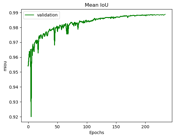
(if save_history=True) is updated and val/train losses and validation
mIOU are plotted in PNG files.
History file description
For each interesting epoch, the training duration (in seconds), the loss on train and validation dataset, the mean IOU on validation dataset and the learning rate are stored.
history file example
{
   "epoch": [0, 1, 2, 3],
   "duration": [697.3998146057129, 630.2923035621643, 333.7448401451111, 170.40402102470398],
   "train_loss": [0.08573817711723258, 0.06264573358604757, 0.059443122861200064, 0.05409131079048938],
   "val_loss": [0.057551397948918746, 0.05338496420154115, 0.049542557676613794, 0.05130733864643844],
   "val_mean_iou": [0.954076948658943, 0.9589184548841172, 0.9638415871794965, 0.9601857738692673],
   "learning_rate": [0.001, 0.001, 0.001, 0.001]
}
Model and optimizer files description
Model and optimizer state_dict are stored as .pth files:
torch.save(self.model.state_dict(), model_file)
torch.save(self.optimizer_function.state_dict(), optimizer_file)
Training plots
Example of plots: